3D Craniofacial Measurement
Cone beam computed tomography (CBCT) is a medical imaging technique consisting of X-ray computed tomography where the X-rays are divergent, forming a cone. CBCT has become increasingly important in treatment planning and diagnosis in implant dentistry, ENT, orthopedics, and interventional radiology (IR), among other things. During dental/orthopedic imaging, the CBCT scanner rotates around the patient’s head, obtaining up to nearly 600 distinct images. For interventional radiology, the patient is positioned offset to the table so that the region of interest is centered in the field of view for the cone beam. A single 200-degree rotation over the region of interest acquires a volumetric data set. The scanning software collects the data and reconstructs it, producing what is termed a digital volume. (Description: © Wikipedia)
This is an outline and brief introduction to investigations in the area of integrated three-dimensional (3D) craniofacial measurement currently in progress at the University of the Pacific School of Dentistry. To demystify some of the underlying principles, we address these questions:
1. Why should orthodontists be interested in 3D craniofacial measurement?
Figure 1. The goal of all orthodontic measurement: a unified craniofacial model. (after Simon)
The goal of craniofacial measurement has always been the re-assembly of information from multiple sources (study casts of the teeth and jaws, x-ray images of the teeth and skull, and photographs of the face) into a common integrated map. Our region of interest, the skull and face, can be considered conceptually to consist of three layers: an overlying soft tissue layer which we image on facial photographs, an underlying array of teeth which we image primarily on study casts, and an intermediate bony layer, the skull and jaws, which is perceivable only on x-ray images.
But the several layers of the skull make it too complex to be grasped as a whole. In the natural state, some layers obscure other layers. For example, from the outside of the mouth, we cannot see the teeth; from the inside of the mouth, we can see the teeth but not the bony armature which supports them. So orthodontists have very cleverly learned to strip away the layers of the system to see the underlying details more clearly. They do this by constructing a series of physical transforms. The usual physical transforms of orthodontics are study casts, cephalometric x-ray images, facial photographs, and panoramic x-ray images. (See Figure 2.)
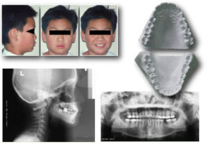
Figure 2. The typical physical transforms of orthodontics.
Each of these transforms, taken by itself, gives us a clearer picture of part of the total system, by completely discarding information about the rest of the system. For example, study casts provide good information about the teeth, but discard all information about the overlying soft issues or the underlying bony scaffolding. Cephalometric x-rays (cephs) provide good information on the scaffold but lose all information about the face surface and retain only attenuated information about the teeth. Facial photographs give us good information about the facial surface, but lose all information about the deeper structures, i.e., the teeth and bones which are perhaps our major concern. Panoramic x-ray images give us valuable information on root contours, but lose all information about arch form and the relationship of the teeth to the facial surface.
However, when orthodontists decompose the skull into separate components, we do not typically retain information on how to put the parts back together with quantitative accuracy. That is why until now the composite illustration from Graber’s text has remained a metaphor —something between a wish and a dream. In current practice, the clinician can do no more than reassemble the information from several transforms conceptually–as a mental operation, in a process called “clinical judgement”. Experienced clinicians do remarkably well at this conceptual task, but with better information we believe that we could deliver even better service to the public.
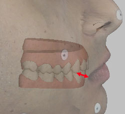
Figure 3a. Measuring between the commissure of the lips and the canine cusp tip.
For example, for purposes of diagnosis and treatment evaluation, we would like to be able to make accurate measurements between physical records of different types (i.e., between study casts and facial photographs, or between study casts and cephalograms). We would like for example to be able to measure precisely how thick the lips are over the canines, how thick the cheeks are over the molars, and what is the relationship between expansion of the maxillary arch and changes in the drape of the buccal soft tissues. Figure 3 attempts to illustrate such relationships, but as may be seen, the very concept is difficult to convey on a two-dimensional image. Information about these and other “tooth to soft tissue” or “tooth to skull” relationships is currently available only for mid-sagittal structures on lateral cephs, and even in that plane the information we have is only marginally trustworthy.
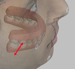
Figure 3b. Measuring between the cheek surface and the buccal surface of the upper first molar.
The problem in making accurate measurements of these kinds is that there is a constraining geometrical law that limits the merging of information from different sources. Although 3D information can be extracted from study casts, conventional facial photographs and x-ray images contain only 2D information. For registration of data from two 2D images it is sufficient to have 2D information for two points that are common to both images. This strategy is used when orthodontists use two “hash marks” to superimpose a pair of lateral cephs. To merge data from two 3D coordinate maps generated from physical records of the same or different kind, one needs to have 3D information (i.e., “x”, “y”, and “z”) for three points common to both maps. This crucial geometric principle will be explored in greater detail later.
In the remainder of this presentation, we will try to outline methods which have now made possible the quantitative re-integration of fully 3D information from different types of physical record.
2. What is the basic principle underlying non-contact 3D measurement from images?
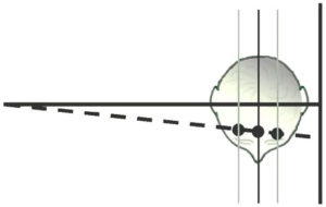
Figure 4.
Conventional lateral and frontal cephs are generated using what is known as projection geometry. The x-rays originating at the focal spot of the x-ray tube radiate such that a small beam collimated near the tube source will cover a progressively larger area the further it is projected from the tube. This phenomenon is well known to orthodontists and is illustrated schematically in Figure 4.
Figure 4 illustrates the path of a single ray from the focal spot on the left through the subject’s head to the film plane on the right. Three planes are drawn, passing through the patient’s head parallel to the film plane but different distances from it. At the point at which the ray strikes the film, information from one point on each para-sagittal plane are “stacked” at the same point demonstrating that the enlargement factor from each plane is different. The distance from each plane to the film represents the “third dimension” for the point on that plane. Only if one knows this third dimension can the point be located uniquely in three dimensional space. The only para-sagittal plane whose distance from the film plane is considered to be known in conventional cephalometry is the mid-sagittal plane itself. This distance is “known” because it is defined by convention as 60 inches in the U.S. and 1500 millimeters in Europe. Also by convention, paired cephalometric landmarks that are positioned lateral to sagittal plane are averaged, a process which ignores the possibility of asymmetry and in any event does not yield a measurement in the third dimension. For unpaired points lying off the sagittal plane or in cases of known asymmetry, no method for estimation of the third dimension is possible on single projection images. However, we can measure the third dimension from 2D projection images if we use the images in pairs, as will now be demonstrated.
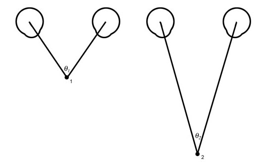
Figure 5a. Natural stereovision. The angle from the left eye to the subject to the right eye varies with the distance to the subject. The closer the subject the larger will be the angle subtended. If one knows the distance between the eyes and the angle to the subject the distance can be calculated with precision. In typical mammalian vision, the viewer performs this operation automatically without being aware of the process unless the subject is so far away that the lines of sight from the two eyes become effectively parallel.
The paradigm for 3D measurement from paried 2D image is taken from nature — from the stereoscopic vision of man and most mammals. It depends on viewing the subject from two different perspectives, which is to say from two eyes located some known distance apart. See Figure 5.
The magnitude of the angle from the left eye to the object being viewed to the right eye is a function of the distance between the viewer and the object viewed. Note that in Figure 5, objects which are further from the viewer will have more acute angles than objects nearer the viewer. Of course, the ability to range the distance to any object from two “eyes” or “cameras” presupposes the ability to identify the same point from both viewing stations.
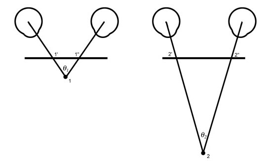
Figure 5b. If a plane parallel to the line between the eyes is interposed between the eyes and the subject, the length of the line segment between the rays from the two eyes will differ proportionally to the difference in the angles. Thus the line segment 1′ to 1″ is a measure of the angle 1 and of the distance between the eyes and point 1. Similarly, the longer line segment 2′ to 2″ is a measurement of the angle 2 and of the distance to point 2.
The application of this principle is the basis for stereoscopic 3D measurement in topographic engineering, cartography, and robotics. In the sections which follow, we demonstrate how it can also be used to make 3D measurements in orthodontics.
References
- Baumrind S, Moffitt FH. Mapping the Skull in 3D. Journal of the California Dental Association 1972; 48:22.
- Baumrind S. A System for Craniofacial Mapping Through the Integration of Data from Stereo X-Ray Films and Stereophotographs. Technical Papers from the Symposium on Close Range Photgrammetric System, American Society of Photogrammetry, University of Illinois, Urbana 1975;142-66.
3. How can one obtain 3D information about structures in the skull from 2D projection images?
In reality, any pair of images in which an object of interest is viewed from two different perspectives can be used to generate 3D information, provided only that 1) the distance between the two viewing points is known and 2) the same point of interest can be seen from both perspectives. In practice, however, certain geometric arrangements between the two viewing perspective and the object of interest have lower error rates than others so that the geometrcial arrangement between viewing stations and the object being measured bear careful consideration. In stereometric measurements of the skull, two different viewing arrangements have been most widely used. These are bi-planar stereometry in which the film casettes for the two exposures are positioned at right angels top each other, and co-planar geometry, in which the two film casettes are oriented parallel to each other. We will consider these in turn.
Bi-planar Stereocephalometry
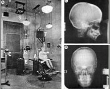
Figure 6a. The original Broadbent apparatus. (From Broadbent, B.H.: Angle Orthodontist 51: 93, 1981.) and a representative Broadbent stereopair.
The first attempts at 3D x-ray cephalometrics by Broadbent 1 and Hofrath 2 retained the most fundamental principle of stereoscopic measurement in that they were based on combining 2D information generated by viewing the subject from two different perspectives. See Figure 6a. Their elegant contributions, while of enormous importance to our specialty, suffered from an unfortunate limitation imposed by the fact that most cranial landmarks have sharply different appearances when viewed from different projections and particularly between lateral and posterio-anterior cephs. Thus there was difficulty meeting the requirement that the same physical point must be located on both images of each stereo-pair. This problem is compounded in the Broadbent geometry by virtue of the fact that the same anatomical landmark typically lies at different distances from the film plane on each of the paired images, as illustrated on Figure 6b.
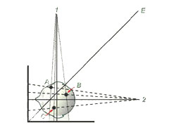
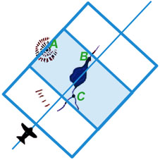
Figure 6b. The geometry of a bi-planar stereopair. Note that each of the three points in the patient’s head (A, B, and C) is located a different distance from the frontal and lateral film planes. For this reason, the points will be enlarged differently on the two films and therefore will have different y coordinates.
Because most landmarks of interest do not lie at the same distance from the film plane on the two images of a Broadbent-Bolton film pair they will have different vertical (y) locations as well as different as well as different horizontal (x) locations. This compounds the problem of locating the same physical point uniquely on both films. Broadbent and his associates attempted to reduce the impact of this problem by constructing a template for matching which they called the Orientator. The use of this device is explained and demonstrated in the accompanying paper presented by Hans and associates.
Co-planar Stereocephalometry
To reduce the difficulty of locating the same physical landmark on both images of a stereopair, our laboratory has for some time been investigating an alternative “co-planar” geometry borrowed directly from photogrammetry and robotics.
First we examine a photogrammetric prototype:
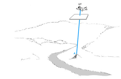
Figure 7a. A mapping aircraft or satellite takes a photograph using a camera pointing straight down. The film plane of the camera is represented schematically below the aircraft. Note that the film plane of the camera is parallel to the surface of the ground. The ray from a point on a hill to the film plane of the camera is shown.
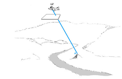 Figure 7b. The plane flies some desired distance and another photograph is taken, again with the camera pointing straight down. The ray from the point on the hill to the repositioned film plane is shown.
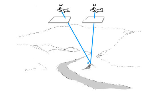
Figure 7c. Figures 7a and 7b are overlayed. Note that this figure precisely analogizes Figure 5b with each position of the aircraft being the equivalent of one eye.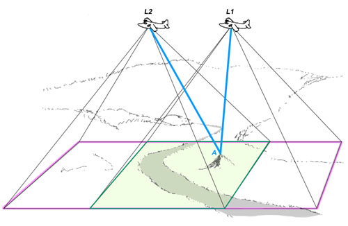
Figure 7d. The region of terrain captured by the camera in each of the two locations is shown. Note that the intersection of rays can only be captured in the area of overlap between the two films.
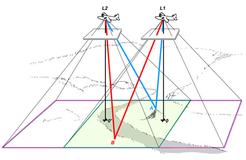
Figure 7e. The analogous intersecting rays to a representative additional point on the ground at the bottom of the hill are shown. Theywill subtend a more acute angle than the rays from the point at the top of the hill. Also, a perpendicular is dropped along the central axis of the camera from each of the two viewing positions. The horizontal distance between the points on the ground directly below the camera is a measure of the distance between thepositions from which the two photographs were taken.
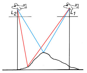
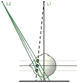
Figure 7f. Schematic two-dimensional representation of Figure 7e. Examine the intersections of the lines with the horizontal film plane; note that the distance between the the blue lines meeting at the top of the hill is less than the distance between the red lines meeting at the bottom of the hill.
At CRIL, we have constructed a co-planar stereocephalometer which uses two x-ray emitters to precisely analogize the geometry of the aerial system in Figure 7 “laid on its side”. See Figure 8a.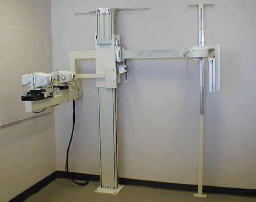
Figure 8a.
A stereocephalometer is shown so oriented that emitter 1 generates a standard cephalogram according to the geometry of the Second Roentgenographic Workshop and yields standard lateral or frontal cephalograms. A second emitter is positioned 18 inches lateral to the first and yields oblique views.
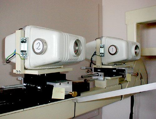
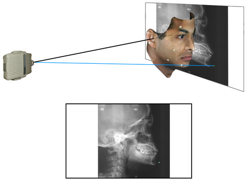
Figure 8c
A schematic representation (not to scale) of a lateral cephalogram. The blue ray (analogous to Figure 7a) passes through a point on the jaw and falls upon the film plane. The path of the central ray along the porion-porion axis is shown.
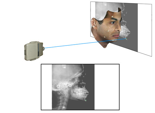
Figure 8d
(Analogous to Figure 7b above) The ray from the second emitter through the same point is shown. Note its point of prejection upon the film plane.
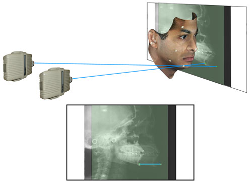
Figure 8e
(Analogous to Figure 7c above) The paths from both emitters through the same point on the chin are shown. The plane view shows both films superimposed. The line connecting the two points on the film plane is a measure of the “height” of the point above the film surface.
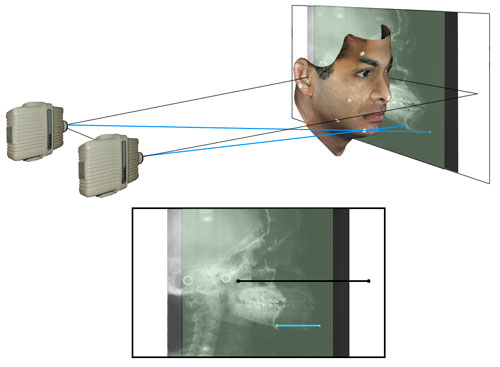
Figure 8f
(Analogous to Figure 7d above) The points on the film plane representing the central rays from both emitters are shown. Note that the black line connecting these two points is an exact measureof the distance between the focal spots of the two emitters.
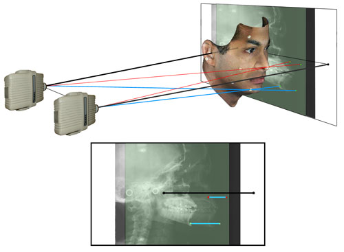
Figure 8g
(Analogous to Figure 7e above) Two additional “red” rays passing through the tip of the nose, a point nearer to the film plane, have been added. Note that the line segment connecting these two points on the film plane is shorter than the segment connecting the blue points. The differences in the lengths of the two line segments is proportional to the heights above the film plane of the nose point and chin point. Note further that the line segments connecting the two images of these and any other point are parallel to the line connecting the focal spots of the emitters.
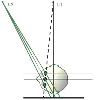
Figure 8h
A schematic top view of the stereocephalometric system (analogous to Figure 7f above). Three points lying on the same ray from the standard emitter but lying at different planes within the skull are shown. Viewed on the single standard lateral cephalogram, these three points would be superimposed on the film plane and their heights would be indistinguishable. However when information from the second emitter is added, it will be noted that the line connecting the two images on the film plane will be of different length, proportional to the heights of the points above the film plane.
A Comparison of Bi-planar and Co-planar Geometries for Craniofacial Mapping
Figure 9a shows the relationship between the two alternative geometries just discussed. Four projection images of the same skull are presented.
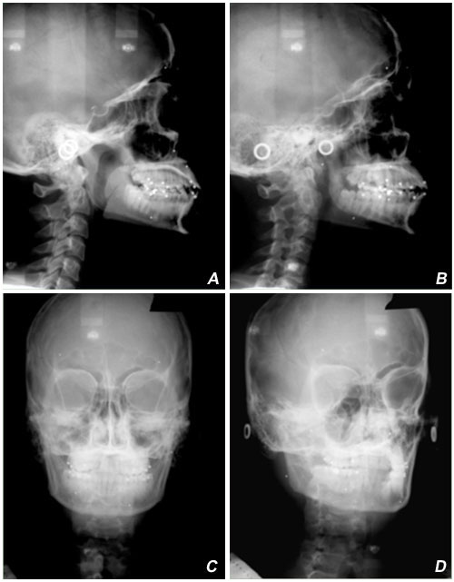
Figure 9a
The upper row constitutes a “coplanar” lateral skull stereopair. “A” shows a conventional lateral ceph taken from Emitter 1 while “b” shows the associated offset lateral ceph taken from Emitter 2. The lower row constitutes the analogous frontal skull stereopair; “C” is a conventional frontal ceph taken from Emitter 1 while “D” is an offset frontal ceph from Emitter 2. The left Column, the stereopair “A” and “C”, constitutes a biplanar, Broadbent-Bolton type stereopair (both of whose images have been generated by Emitter 1).
An examination of these four component images of Figure 9a demonstrates dramatically that it is much easier to locate the same anatomical structure on the two images of a coplanar stereopair (say, for example, sella or pogonion on “A” and “B”) than it is to locate the same anatomical structure on both images of the biplanar steropair, “A” and “C”. This is true mainly because the image of any given structure changes less between the two views of a coplanar pair than it does between the two views of a biplanar steropair. But there is an important additional reason why locating the same anatomical structure on a biplanar stereopair is more difficult than it is on a coplanar stereopair. This is because there is an important additional clue for checking that one has located the same structure on both images of the steropair which do not exist in the biplanar case.
Recall that for a biplanar pair, one locates the “x” and “y” positions of a point on the lateral ceph and its “y” and “z” positions on the frontal ceph. At first glance, one might think that an important clue for checking that you have indeed located the same physical point on both images would be that the “y” coordinates on both images would be the same. (Indeed this appears to be what at least some of Broadbent’s co-workers originally believed.) Unfortunately, this assumption is incorrect as may be seen in Figure 9b.
 |
 |
| Figure 9b | Figure 9c |
Here it may be seen that each of the three points in the skull (represented by A, B. and C) is located a different perpendicular distance from the surfaces of the frontal and lateral film surfaces. This means that the paired images of each point will fall on different heights (i.e., have different “y” coordinates) on the frontal and lateral film surfaces. In fact, only points lying along the bisecting plane represented by the line E in Figure 9b will have the same “y” coordinate on both the lateral and fronatal cephs of a Broadbent-Bolton stereopair. Indeed, this is precisely the problem that Broadbent’s “Orientator” sought to correct, although the method was a bit too cumbersome in practice to ever catch on.
A much simpler alternative is available in coplanar systems where, as may be seen in Figure 9c, the perpendicular distance from each point in the skull to the film surface is automatically the same for both films of any stereo pair.
For this reason, correlation of the two images of the same point or structure on co-planar stereo pairs is further simplified as is demonstrated in Figure 9d.
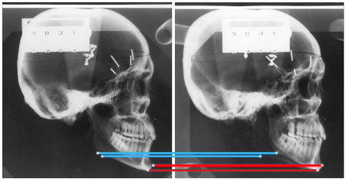
Figure 9d
Here we see co-planar lateral ceph images of a dried skull with metal markers at left and right gonion and also at pogonion or menton. The pairing of the poginion and menton points on the centered and offset lateral images is quite straightforward, because we can easily tell menton from pogonion on each of the two different views considered separately. But how do we keep from confusing the images of right and left gonion on the two images. Indeed, they look remarkably similar!
The answer lies in the geometrically determined fact that each structure has the same “Y” coordinate on both the centered and the offset image. For this reason we need only link the upper image of gonion on one image with the upper image of gonion on the other image; (similarly, lower with lower). In the stereo pair shown, the longer gonion-gonion line (i.e., the upper line) represents the side near the x-ray source, while the shorter gonion-gonion line represents the side further from the x-ray source and nearer to the film plan. Note that the poginion-pogonion line and the menton-menton line are of equal length because they both lie the same distance from the film plan.
For points not unambiguously identifiable this “Y to Y” correspondence is a powerful error control mechanism; if the y coordinate of any given point is not the same on both the centered and offset images, it has been misidentified on at least one of the images.
References
- American Journal of Orthodontics 1983;84:292-312.
- Baumrind S, Moffitt FH, Curry S. The Geometry of Three-Dimensional Measurment from Paired Coplanar X-Ray Images. American Journal of Orthodontics 1983;84:313-22.
4. How is 3D information about the surface of the face obtained?
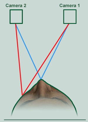
Figure 10a. Ranging the location of two representative points on the face from a pair of cameras located a known distance apart.
The task of generating 3D information about the facial surface is conceptually no different from that outlined above for terrestrial and x-ray photogrammetry as may be seen in Figure 10a (compare to Figures 7f and 8h).
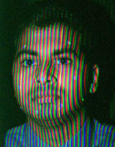
However, whereas in stereocephalometry it is still necessary to locate each point of interest manually on both images of a stereo pair, recent advances in imaging technology now make it possible to assemble 3D surface maps of the face fairly automatically. These methods utilize technologies known collectively as “structured light imaging.” Briefly stated, they involve projecting a known grid or similar image on the facial surface from one perspective and then photographing the distortion of the projected image with a single camera whose spatial location is known with respect to the location of the projector. The general method of projecting a grid on a subject to be mapped has been known for many years but was not considered practical for clinical use earlier because locating large numbers of grid intersections by hand, even on a single image, was prohibitively labor-intensive. This objection is now overcome in a number of structured light systems. In general, vertically oriented series of rainbow stripes is projected on the subject by a specialized projector and then photographed by a digital camera located a known distance from the projector.
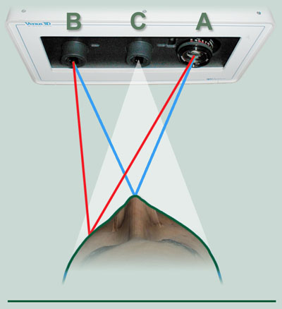
Figure 10b. In a more recent development, a second digital camera (C), mounted between the fixed projector (A) and digital camera (B) captures a true-color image a few milliseconds after the primary image.
A known pattern is projected upon the subject from a light source (A) and photographed by a digital camera (B). See Figure 10b. The 3D information from the primary-camera-light-projector assembly is synchronized with the 2D pixel map from Camera C and is stored in a kind of look-up table. In this way, the location of each pixel on the monitor-displayed image from Camera C uniquely identifies the three dimensional coordinates of a particular point on the surface map generated by Camera B and its associated projector (A).
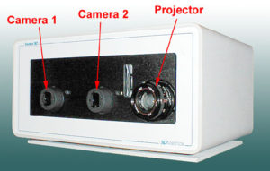
Figure 10c. The 3D Metrics Camera System currently in use at CRIL.
A camera system utilizing this approach (manufactured by 3D Metrics, Petaluma, California) is shown in Figure 10c. In this implementation, one of the usual cameras of the stereo pair is replaced by a light projector which casts a grid-like pattern or array upon the subject from a known location and orientation. A dedicated computer chip built into the digital camera has the ability to distinguish different frequencies of light and hence can tell, from the color of each light ray, the direction in which that particular ray has traveled from the light projector.
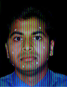
Figure 10d.
Figure 10e.
The projected pattern falling upon the subject is photographed by Camera 1 which is mounted a known distance from the Projector. When viewed from the perspective of the Projector, the shape of the projected pattern remains unaltered regardless of the shape of the object it falls upon (see Figure 10d).
When viewed from the perspective of Camera 1, the projected pattern is distorted as a function of the height of the various features of the subject’s face (see Figure 10e). Since the view of the pattern from the vantage point of the projector is always an unaltered representation of the pattern itself, it need not be digitized at each exposure. Instead, the heights of the various facial features can be calculated solely from the distortion of the pattern when viewed from the vantage point of Camera 1.
The reconstructed representation of the face can be rotated on a standard computer monitor and the 3D coordinates of any visible point can be captured by pointing and clicking with a standard mouse or other similar device (see Figure 10f).
Figure 10f.
5. How is 3D information about tooth size and arch form obtained?
The structured light methods just described are quite sufficient to locate landmarks to an accuracy of about one millimeter on the surface of the face. However, they are not capable at this time of the greater accuracy required for more detailed automated measurement of tooth surfaces. Additionally, like all photographic measurements, they are subject to “line of sight” problems which means that they cannot see around undercuts. For the greater accuracy required to make detailed maps of structures with multiple undercuts (like orthodontic study casts), alternative methods are required. Perhaps the best of these currently available for our purposes is the technique of “destructive scanning.” Destructive scanning is a one of a number of methods used in engineering to assess the quality of electronic circuits by slicing them into component layers. By disassembling, testing, and inspecting a device, a complete profile can be created to determine how well a device conforms to design and process requirements.
For biologically trained observers like orthodontists, perhaps the best analogy for understanding destructive scanning is the “serial section” which we all remember from our earlier studies of histology and pathology. Recall that when we want to understand the 3D structure of a block of tissue in those disciplines, we invest the block after suitable preparation in a material of matched cutting properties and then make a series of slices with a microtome. The surfaces of the slices are then examined sequentially under a microscope and a 3D picture is constructed by mentally comparing the appearance of slices which lay and different depths into the block. In the destructive scanning of dental study casts, a carefully fabricated white stone cast is invested in black epoxy plastic of similar cutting properties. After the epoxy has set, the surface of the block is cut or milled until the first trace of white study cast appears. At that point, the 2D surface of the block is scanned with a flying spot laser scanner and the limits of the outline of the area of white study cast are mapped and stored in the computer. The entire surface of the block is then milled to a depth of approximately three thousands of an inch (~0.1 mm) and the process of laser scanning and 2D mapping is repeated. This process of slicing and mapping is repeated until the entire tooth-bearing portion of the cast has been milled and mapped. In place of a physical study cast, we now have a series of stackable computer stored 2D outlines from which a 3D virtual map of great accuracy can be generated as desired. Note that this method of serial slicing and scanning completely eliminates the undercut problem which is such a major issue in many dental applications.
The resulting virtual 3D map can be represented on a computer screen. (See Figure 11a.)
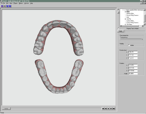
Figure 11a
The virtual study casts can be manipulated, measured, or modified as desired on screen through the use of specialized software. Also, if desired, the virtual models can be used to regenerate physical 3D replicas of the original or of some desired modification of the original) using another new technology called stereolithography.
Stereo-lithography (SLA) is one of a number of new technologies for constructing 3D physical models from virtual 3D digital maps stored in computers. It uses a photo-curable liquid resin (either epoxy, vinyl-ether, or acrylate) which has the property of solidifying or “curing” when exposed to an ultra-violet beam from a HeNe (helium-neon) laser. The laser can be moved and positioned over a pool of the photo-curable liquid under the control of a computer file such as the 3D coordinate map previously generated during the course of the destructive scanning process described above. Thus, stereo-lithography offers us the ability to reconstruct a physical three-dimensional object from the virtual 3D computer map.
The process is illustrated schematically in Figure 11b.
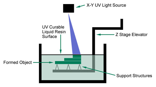
Figure 11b
A vertically operating elevator is suspended in a tank of photo-curable liquid resin such that a support for the 3D object to be re-created lies slightly below the surface of the liquid. Under computer control, the laser then scans onto the surface of the liquid, the shape of the apical-most slice of the virtual study cast model. This causes a thin slice of the liquid resin to congeal. The elevator is now lowered .0003 inch deeper into the liquid bath and the laser scans the next digital layer of its virtual model onto the resin bath, causing the second layer to congeal. The chemical properties of the resin are such that the sequenced layers of congealed resin bind to each other spontaneously. The elevator is lowered another .003 inch and the laser scanning process is repeated. This series of steps is iterated until a solid plastic representation of the original study cast is created.
Although both technologies have become practical only in the last decade, variants of destructive scanning and stereolithography are already used in many industries. Among their most rapidly growing applications is that in orthodontics where they are employed for different applications by both Invisalign and Orthocad, We wish to thank the Invisalign Corporation for its considerable assistance in developing the CRIL application that we report here.
6. How do we merge 3D maps of the skull, face, and teeth?
The final task is the merging of data from different 3D digital maps. The conceptual basis for merging is again an idea adapted from terrestrial photogrammetry. In that domain, it is frequently desirable to merge data from overlapping 3-dimesional maps generated by aircraft or satellites surveying targets from different directions and altitudes. Figure 12 illustrates schematically the rationale for such an operation.
 |
 |
| Figure 12a | Figure 12b |
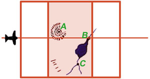
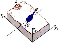
Detail 12a shows in plan view an aircraft taking an overlapping stereo pair of images while flying over the terrain from left to right. The region of overlap of the two images of the stereo pair, shown here shaded in red, is called the “neat” region and is analogous to the overlapping regions of Figures 7d and 7e, and also of Figures 8f and 8g. From information contained in this neat region, the 3D model shown in Detail 12b can be constructed. Note that three unambiguous landmarks—A, B, and C—have been located in the region of overlap in Detail 12a and have accordingly also been identified in the 3D model shown in 12b.
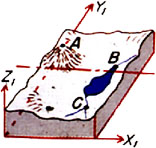
At a different time, a second aircraft flying over the terrain from a different direction generates another stereo pair of images (Detail 12c) from which a second 3D model can be constructed (Detail 12d).
 |
 |
| Figure 12c | Figure 12d |
Because the two stereo pairs were generated from different perspectives they and the 3D models generated from them do not overlap completely. However, they and the two 3D models generated from them do share in common three unambiguous landmarks: A, B, and C. If the two 3D models could be rotated and translated through space until their paired images of A, B, and C could be brought into consonance, the neat areas of the two stereo pairs could be merged to yield a continuous 3D model. A plan view of such a model is shown in Detail 12e with the neat portions of the two stereo pairs overlapping and continuous.
 |
| Figure 12e. (Please note: this is an animation. If the points aren’t blinking, check your browser’s settings to make sure that animated GIFs play continuously.) |
At this point any landmark unambiguously identifiable on one 3D model can be precisely related to any point unambiguously identifiable on the other model. Two such points are represented by the red and blue blinking points in Figure 12e.
In many terrestrial mapping situations (for example, in desert areas), few or no unambiguous markers like A, B, and C common to 2 or more stereo pairs exist in the terrain. In such cases, artificial markers, called “tie points” are placed on the ground before the overflight in which the stereo images are generated.
An analogous situation exists in craniofacial imaging. Therefore we take a leaf from photogrammetrists and from the work of Bjork, and add our own unambiguous metal markers. But in this case we fasten the tie points only temporarily to the surfaces of the teeth and face. Such an application is presented in the section on Clinical Implementation which follows.
7. Clinical Implementation
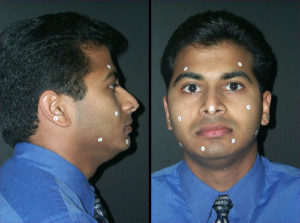
Figure 13a.
In our current implementation, an accurate poly vinyl siloxane (PVC) impression of each arch is obtained and stereo-lithographic models of the upper and lower dentitions are generated in the laboratory using the methods described above. Conventional pull-down overlay retainers are fabricated on the stereo-lithographic casts with radiopaque metal spheres replacing their resin precursors on the SLA models. The overlay appliances are inserted in the mouth and their occlusal interferences are adjusted (Figure 13b). A hard wax checkbite is generated in centric relation. Additional triads of radiopaque markers are affixed to the surface of the face (Figure 13a) and images of the face are generated using the specialized 3D camera. Lateral and frontal x-ray stereopairs (Figure 13c) are generated with the apparatus shown in Figure 8 using the DenOptix digital image capture system.
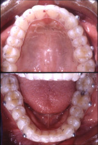
Figure 13b.
The 3D coordinates of the radiopaque tie points are located (at high precision and in replicate) on each the several images. Those on the facial images are located from the 3D camera images projected directly upon a conventional computer monitor (see Figure 10f). Those on the study cast tie points have been quantified earlier during the process of destructive scanning, SLA fabrication, and overlay retainer construction. The coordinates of all landmarks visible on the digital x-ray images are located separately on each image of each stereo pair using on-screen variants of previously developed 2D methods for locating landmarks on x-ray images 16. Finally, using software constructed to our specifications, the coordinates of all tie points on all images are merged into a unified 3D data set and a computer graphics program carries along available contour information on the tooth, bone, and facial soft tissue surfaces in proper orientation.
The output of these operations is an integrated 3D coordinate map of the multiple layers of the skull and face that can be displayed, manipulated, and measured as desired on a conventional computer monitor. The several movies which follow are examples of integrated craniofacial maps generated using the methods outlined above.
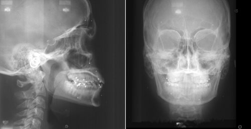
Figure 13c.
References
- Baumrind S, Moffitt FH. Mapping the Skull in 3D. Journal of the California Dental Association, 1972; 48:22.
- Baumrind S. A System for Craniofacial Mapping Through the Integration of Data from Stereo X-Ray Films and Stereophotographs. Technical Papers from the Symposium on Close Range Photgrammetric System, American Society of Photogrammetry, University of Illinois, Urbana, 1975; 142-66.
- Baumrind S, Moffitt FH, Curry S. Three-Dimensional X-Ray Stereometry from Paired Coplanar Images: A Progress Report. American Journal of Orthodontics, 1983; 84:292-312.
- Baumrind S, Moffitt FH, Curry S. The Geometry of Three-Dimensional Measurment from Paired Coplanar X-Ray Images. American Journal of Orthodontics, 1983; 84:313-22.